How to perform data augmentation and clean your dataset with fastai

In this blog post, I’ll be showing you how you can implement data augmentation and how you can clean you data after training your model to improve your model’s performance. These techniques were discussed in Lesson 2 of the fast.ai course and in Chapter 2 of the fastbook. We’ll be continuing on from the previous post and using the Iron Man suit classifier that we built earlier. The initial set-up will be identical to the set-up in the previous post.

Initial Set-up:

!pip install -qq git+https://github.com/rwightman/pytorch-image-models
!pip install -Uqq fastai
!pip install -Uqq fastbook
# import gradio as gr
from fastbook import *
from fastai.vision.widgets import *
from fastai.vision.all import *

# If you want to try out other architectures:
!pip install -Uqq timm
!pip install git+https://github.com/rwightman/pytorch-image-models.git
import timm

# code to handle issue with VSCode Jupyter extension not printing epoch results:
from IPython.display import clear_output, DisplayHandle
def update_patch(self, obj):
    clear_output(wait=True)
    self.display(obj)
DisplayHandle.update = update_patch

from fastdownload import download_url

class_1 = 'iron man mark 1'
save_class_1 = class_1 + '.jpg'
class_2 = 'iron man mark 2'
save_class_2 = class_2 + '.jpg'
class_3 = 'iron man mark 3'
save_class_3 = class_3 + '.jpg'
class_4 = 'iron man mark 4'
save_class_4 = class_4 + '.jpg'

download_url(search_images_ddg(class_1, max_images=1)[0], save_class_1, show_progress=False)
Image.open(save_class_1).to_thumb(256,256)

download_url(search_images_ddg(class_2, max_images=1)[0], save_class_2, show_progress=False)
Image.open(save_class_2).to_thumb(256,256)

download_url(search_images_ddg(class_3, max_images=1)[0], save_class_3, show_progress=False)
Image.open(save_class_3).to_thumb(256,256)

download_url(search_images_ddg(class_4, max_images=1)[0], save_class_4, show_progress=False)
Image.open(save_class_4).to_thumb(256,256)

searches = 'iron man mark 1', 'iron man mark 2', 'iron man mark 3', 'iron man mark 4'
path = Path('iron_man_suit_classifier')
from time import sleep

for o in searches:
    dest = (path/o)
    dest.mkdir(exist_ok=True, parents=True)
    download_images(dest, urls=search_images_ddg(f'{o}'))
    sleep(10)  # Pause between searches to avoid over-loading server
    download_images(dest, urls=search_images_ddg(f'{o} photo'))
    sleep(10)
    # download_images(dest, urls=search_images_ddg(f'{o}'))
    # sleep(10)
    resize_images(path/o, max_size=400, dest=path/o)

failed = verify_images(get_image_files(path))
failed.map(Path.unlink)
len(failed)

suits = DataBlock(
    blocks=(ImageBlock, CategoryBlock), 
    get_items=get_image_files, 
    splitter=RandomSplitter(valid_pct=0.2, seed=42),
    get_y=parent_label,
    item_tfms=[Resize(192, method='squish')]
)
dls = suits.dataloaders(path)
dls.train.show_batch(max_n=8)

Data Augmentation

Data augmentation is used to create random variations of a dataset without changing the meaning of our data to increase the diversity and size of the dataset. Variations made to our data could include flipping, resizing and cropping of our images. By presenting the neural network with random variations of the same image, it will have more training opportunities with the image which helps the model understand what the object is.

We’ll be using the aug_transforms function and passing it through the batch_tfms parameter to tell fastai that we want to perform these transformations on an entire batch of our data. After creating our DataBlock object - this is where we’ll implement data augmentation. Once we have augmented our dataset, we’ll need to reload our data using dataloaders.

# transform our data using RandomResizedCrop and aug_transforms:
suits = suits.new(
    item_tfms=RandomResizedCrop(224, min_scale=0.5),
    batch_tfms=aug_transforms()
)
# reload our data:
dls = suits.dataloaders(path)
dls.train.show_batch(max_n=10, unique=True)

Your output should look something like this:

Here, we can see that slight random variations have been applied to one of the images in our training set. Now, let’s train our model again with our dataset that has had data augmentation performed.

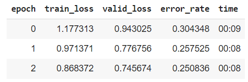
learn = vision_learner(dls, resnet18, metrics=error_rate)
learn.fine_tune(3)

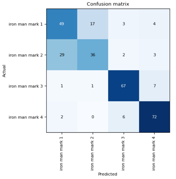
interp = ClassificationInterpretation.from_learner(learn)
interp.plot_confusion_matrix()

plt.rcParams.update({'font.size': 8})
interp.plot_top_losses(5, nrows=1)

OK, our training performance did slightly worse than the performance we achieved in our previous post. However, note that we did have to re-search and re-download all of the images used in our training annd validation set in this post so it makes sense that our training results are quite different. We were able to achieve an accuracy of 72%, which is adequate but could certainly be improved. Let’s see if we can improve our accuracy by cleaning our data.

Based on the confusion matrix results, we can see that our model had a lot of difficulty correctly classifying images of the Mark 1 and Mark 2 classes. This makes sense the two classes look similar in colour. Let’s use ImageClassifierCleaner to clean our datasets.

from fastai.vision.widgets import *
cleaner = ImageClassifierCleaner(learn)
cleaner

Your output should look something like:

Here, you’ll want to re-classify any images that shouldn’t be in the current class that you’re looking at and delete the image if it doesn’t fall into any of your classes. Once you have made these changes, run the below code and then repeat this process for all the different training and validation sets per class. Remember to run the below code after each change you make.

# To delete all images selected for deletion:
for idx in cleaner.delete(): cleaner.fns[idx].unlink()
# To move images into a different selected category:
for idx,cat in cleaner.change(): shutil.move(str(cleaner.fns[idx]), path/cat)

Once you have finished cleaning you data, reload the data and then train your model again using your newly cleaned dataset.

dls = suits.dataloaders(path)
learn = vision_learner(dls, resnet18, metrics=error_rate)
learn.fine_tune(3)

interp = ClassificationInterpretation.from_learner(learn)
interp.plot_confusion_matrix()

Our results show a slight increase in training accuracy but we can see from the confusion matrix that our model is still finding it very challenging to distinguish between the Mark 1 and Mark 2 images. As we saw from the ImageClassifierCleaner GUI, a lot of the images in our training and validation set is very poorly labelled, hugely affecting our training results. Perhaps an Iron Man suit classifier wasn’t the best example to show you effectiveness of our image classification process… but I hope you get the gist anyway!

Resources