How to train and deploy a simple model using fastai.
In this blog post, I’ll be showing you how to leverage the fastai library to train a simple deep learning model and deploy it as a web app using Gradio. This post is based on Lesson 2 of the fast.ai course - to watch the online lecture video that was recorded for this lesson at UQ in 2022, go here. To check out the corresponding chapter in the Practical Deep Learning for Coders with fastai & PyTorch, go here. This was a really cool lesson in the fast.ai course where Jeremy walks you through the process of building your own image classification model, how to perform data augmentation and clean up your data after training your model to improve your model’s accuracy, and how to deploy your model as an interactive web app. This lesson is super practical and fun - which is was why I chose to document my experience playing around with my own model and to show you how simple the process can be using the fastai library!
Let’s build an Iron Man suit classifier!
Step 0. Set-up your environment.
I built my image classifier model and app using the VSCode Jupyter extension in GitHub’s CodeSpaces. However, you could you just create a notebook in Kaggle, Google Colab or Jupyter Notebook (via Anaconda). Now, let’s first install and import all the necessary libraries we’ll need to train and deploy our deep learning model:
!pip install -Uqq fastai
!pip install -Uqq fastbook
import gradio as gr
from fastbook import *
from fastai.vision.widgets import *
from fastai.vision.all import *
If you’d like to play around with multiple other deep learning architectures that don’t already come with the fastai library, import timm as well:
# If you want to try out other architectures:
!pip install -Uqq timm
!pip install git+https://github.com/rwightman/pytorch-image-models.git
import timm
If you are also using the VSCode Jupyter extension to run your Jupyter notebook, you may also be affected by a bug that will prevent your fine-tuning results to print. If that’s the case, run this code snippet to fix that issue:
# code to handle issue with VSCode Jupyter extension not printing epoch results:
from IPython.display import clear_output, DisplayHandle
def update_patch(self, obj):
    clear_output(wait=True)
    self.display(obj)
DisplayHandle.update = update_patch
Alright, in my experience trying to run Jeremy’s “is it a bird” image classifier example from Lesson 1, the DuckDuckGo search API had a bug that prevented the notebook from running smoothly. Let’s just run this snippet of code to make sure that our search images function is working:
# Code to test if search_images_ddg is working:
from fastbook import *
urls = search_images_ddg('grizzly bear', max_images=100)
len(urls),urls[0]

download_url(urls[0], 'images/bear.jpg')
im = Image.open('images/bear.jpg')
im.thumbnail((256,256))
im
OK - if that’s all working, then we can start building!
Step 1. Create our testing dataset.
The first step is to download some images that you can load into your image classifier app later to test out your model. For my example, I’d like to build and train a model to classify different Iron Man suits. So I’ll be downloading images of the four different Iron Man suits I’d like to classify.
from fastdownload import download_url

class_1 = 'iron man mark 1'
save_class_1 = class_1 + '.jpg'
class_2 = 'iron man mark 2'
save_class_2 = class_2 + '.jpg'
class_3 = 'iron man mark 3'
save_class_3 = class_3 + '.jpg'
class_4 = 'iron man mark 4'
save_class_4 = class_4 + '.jpg'

download_url(search_images_ddg(class_1, max_images=1)[0], save_class_1, show_progress=False)
download_url(search_images_ddg(class_2, max_images=1)[0], save_class_2, show_progress=False)
download_url(search_images_ddg(class_3, max_images=1)[0], save_class_3, show_progress=False)
download_url(search_images_ddg(class_4, max_images=1)[0], save_class_4, show_progress=False)

# you may want to run the following lines in separate code cells in your notebook so that you can inspect each image individually:
Image.open(save_class_1).to_thumb(256,256)
Image.open(save_class_2).to_thumb(256,256)
Image.open(save_class_3).to_thumb(256,256)
Image.open(save_class_4).to_thumb(256,256)
Step 2. Create our training and validation dataset.
Now, we are going to search for and download images for each of the classes that we want to train our model to classify. This block of code will also save the images in labelled folders in the given path directory based on their class name - which will give the images their corresponding labels.
searches = 'iron man mark 1', 'iron man mark 2', 'iron man mark 3', 'iron man mark 4'
path = Path('iron_man_suit_classifier')
from time import sleep

for o in searches:
    dest = (path/o)
    dest.mkdir(exist_ok=True, parents=True)
    download_images(dest, urls=search_images_ddg(f'{o}'))
    sleep(10)  # Pause between searches to avoid over-loading server
    download_images(dest, urls=search_images_ddg(f'{o} photo'))
    sleep(10)
    # download_images(dest, urls=search_images_ddg(f'{o}'))
    # sleep(10)
    resize_images(path/o, max_size=400, dest=path/o)
Before we start training our model, we’ll want to remove any images that failed to download correctly.
failed = verify_images(get_image_files(path))
failed.map(Path.unlink)
len(failed)
Now, in order to load our dataset (the downloaded images) into our model, we’ll first need to create a DataBlock. More information on what a DataBlock is can be found in Lesson 1’s Kaggle notebook and in fastai’s docs.
suits = DataBlock(
    blocks=(ImageBlock, CategoryBlock),
    get_items=get_image_files,
    splitter=RandomSplitter(valid_pct=0.2, seed=42),
    get_y=parent_label,
    item_tfms=[Resize(192, method='squish')]
)
dls = suits.dataloaders(path)
dls.train.show_batch(max_n=8)
Your output should show a sample batch of the images in your training set and should look something like this:

Step 3. Train our model.
We can finally start training our model - yay! For this example, we’ll train our model using the resnet18 CNN architecture, use error rate as our metric, and train for 3 epochs.
learn = vision_learner(dls, resnet18, metrics=error_rate)
learn.fine_tune(3)
learn.loss_func
Once the model has finished training all epochs, the output should show the results of the training like this:

We were able to achieve roughly 77% accuracy after 3 epochs - which is not bad but it certainly could be better! To better understand why our model could be underperforming, let’s see if we can get more insight into our training results.
Running the below code will give us a matrix of the images used to validate our model and what the model predicted. The top line reveals the ground truth and the bottom line shows the prediction that the model made.
learn.show_results()
")
From this, we can start to see where the model got confused… it looks like it had a bit of a hard time distinguishing between Iron Man Mark 1 and Mark 2 suits. Let’s get some more information on our training results. Let’s plot a confusion matrix to gain a better understanding of what our model found challenging to classify.
interp = ClassificationInterpretation.from_learner(learn)
interp.plot_confusion_matrix()
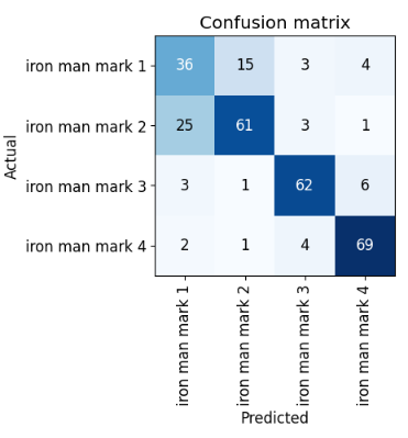
Interestingly, we can see that most of the prediction mistakes were made on the Mark 1 and Mark 2 classes… which kind of makes sense, because they are quite similar in colour. Also, we can also see that there were considerably fewer images of the Mark 1 suits in our dataset. This might have affected our model’s training performance in learning about the differences between Mark 1 and Mark 2.
If we want to gain more information on our model’s training performance, we could also plot the top losses and predictions it made using:
interp.plot_top_losses(5, nrows=5)
But based on the results, we can see how important it is that our training and validation datasets need to be high quality. We also need to make sure that our model has enough images to train on, particularly when some of the classes are very similar and hard to distinguish between.
Step 4. Deploy our model.
Now, let’s deploy our model into a web application using Gradio. Frist, we’ll need to export and save our model so that it can be loaded into our prediction function.
learn.export()
# Let's check that the file exists, by using the ls method that fastai adds to Python's Path class:
path = Path()
path.ls(file_exts='.pkl')
Now, let’s load our model:
learn = load_learner('export.pkl')
Let’s define a prediction function for our model:
labels = learn.dls.vocab
def predict(img):
    img = PILImage.create(img)
    pred,pred_idx,probs = learn.predict(img)
    return {labels[i]: float(probs[i]) for i in range(len(labels))}
Now, let’s make a Gradio interface to run our web app with:
# Customizing Gradio app:
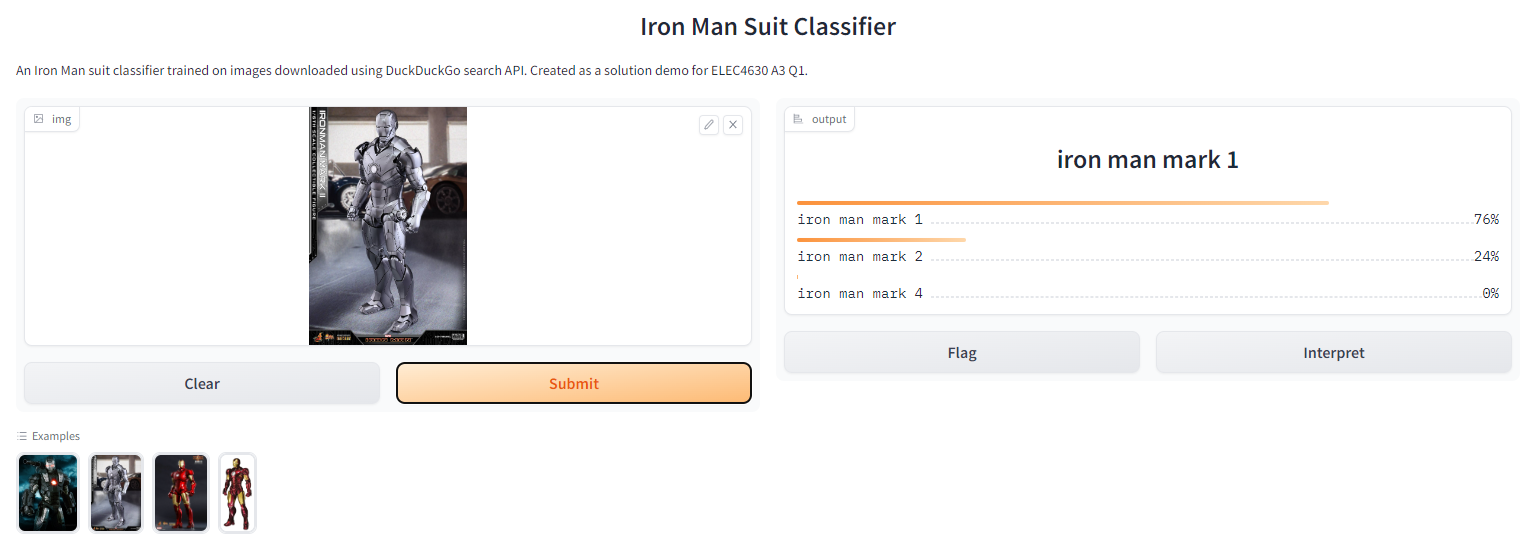
title = "Iron Man Suit Classifier"
description = "An Iron Man suit classifier trained on images downloaded using DuckDuckGo search API. Created as a solution demo for ELEC4630 A3 Q1."
examples = [save_class_1, save_class_2, save_class_3, save_class_4]
interpretation='default'
enable_queue=True
gr.Interface(fn=predict,inputs=gr.inputs.Image(shape=(512, 512)),outputs=gr.outputs.Label(num_top_classes=3),title=title,description=description,examples=examples,interpretation=interpretation,enable_queue=enable_queue).launch(share=True)
There should be two URLs in our output from which we can launch our Gradio web app. Let’s click on one of them and try out our web app:
 There you go - you have just created your very own image classifier web app!
I hope you’ve had just as much fun as I have in building this :)
Resources
- Lesson 2 of the fast.ai course: https://course.fast.ai/Lessons/lesson2.html
- Relevant book chapter: https://github.com/fastai/fastbook/blob/master/02_production.ipynb
- Tutorial on using Gradio: https://www.tanishq.ai/blog/gradio_hf_spaces_tutorial
- fastai docs: https://docs.fast.ai/